Gamma Knife is a well-established radiotherapy treatment system specifically designed to treat intracranial brain lesions. One of the main advantages of Gamma Knife stereotactic radiosurgery (SRS) is its precision, enabling the clinicians to deliver very high doses in a single fraction. The first Gamma Knife device using cobalt-60 (⁶⁰Co) radioisotope was introduced by Lars Leksell in 1967 [1–5]. Since then, several models such as U, B, C, and Perfexion have been developed for stereotactic radiosurgery [4,6–8]. The latest system, Leksell Gamma Knife (LGK) Icon (Elekta Instruments AB, Stockholm, Sweden) with an onboard cone-beam computed tomography (CBCT) imaging system, utilizes 192 ⁶⁰Co sources to deliver collimated radiation beams to target areas with high accuracy [9,10]. The sources are fixed inside eight independent moveable sectors, with each sector containing five rings and 24 sources per sector. Each sector can be aligned with one of three collimator sizes (4, 8, or 16 mm) or blocked if the sector is not required for treatment. The collimators are designed to focus the radiation from the individual sources on to a common point in space, referred to as the focus position. An SRS treatment with LGK is characterized by a combination of various sector, collimator, and couch positions referred to as shots. A Gamma Knife treatment is based on one or more shots; each shot is characterized by its location in stereotactic space, collimator size (independently set per sector), and contribution to the overall target dose (weight). The shot parameters and their distribution are determined during treatment planning by clinicians. The irradiation time (shot time) required to deliver the prescribed target dose is calculated by accounting for the radioactive decay of the sources and the radiation attenuation properties of various cranial tissue.

Treatment accuracy can be attained with a stereotactic frame rigidly attached to the patient’s head or a specially designed thermoplastic mask with infrared markers for high definition motion management (HDMM) system during treatment. Computed tomography (CT), magnetic resonance imaging (MRI), and angiography are image modalities commonly used in treatment planning.

The onboard CBCT imaging system of the LGK Icon uses an air-cooled X-ray tube with an energy range of 70–120 kV_p and a focal spot size of 0.6 mm. The detector consists of a CsI layer and an amorphous silicon thin-film transistor (a-Si TFT) array. Icon can reconstruct imaging volumes of 224 mm × 224 mm × 224 mm with a pixel size of 0.368 mm and a magnification of 1.27. The scan time is typically 30 seconds. Fig. 1 shows a schematic of the LGK Icon CBCT. As the detector is close to the object being scanned, a large proportion of the scattered radiation reaches the detector plane, thereby degrading the image quality. Due to the physical design constraints of the system needed for clearance, the CBCT system is unable to sample data from all angles around the patient with a scanning arc of 200° used for all patients. This results in cone-beam artifacts during image reconstruction, including the appearance of smeared-out structures at the top of the head [11].

The Icon CBCT acquisition offers a choice between two preset modes: a high dose preset (6.3 mGy per scan) for treatment planning simulation scans and a low dose preset (2.5 mGy per scan) for pre-treatment image guidance. Other parameters, including energy (90 kV_p), gantry start and stop angles, and field-of-view (FOV), are not variable. Customer acceptance tests of the CBCT system include image quality (spatial resolution, contrast-to-noise, and uniformity) measured with a CatPhan 503 (The Phantom Laboratory, New York, NY, USA) and CBCT precision (treatment and CBCT isocenter coincidence) measured with the QA Tool Plus (Elekta Instruments AB). Commissioning tests also included dosimetry (kV_p and CTDI) measured with an Unfors RaySafe X2 detector system (Unfors RaySafe AB, Billdal, Sweden), geometric accuracy measured with the CatPhan, and image registration accuracy measured using fiducial markers on a STEEV phantom (CIRS, Norfolk, VA, USA). The routine quality assurance protocol for the Icon involves daily measurements of coincidence between the imaging and treatment isocenters, to within a tolerance of 0.4 mm with typical measurements less than 0.2 mm. In addition, CBCT image quality (uniformity, spatial resolution, contrast to noise, and geometric accuracy) is verified monthly against manufacturer specifications, as is CBCT dosimetry (CTDI and energy) which is measured biannually.

Dose calculations are performed with Leksell GammaPlan (LGP), using either a simple homogeneous dose algorithm known as TMR10 or a convolution dose algorithm [12,13]. The convolution algorithm accounts for differences in relative electron density data derived from patient CT datasets acquired prior to treatment. In this study, we examine the feasibility of using the onboard CBCT for deriving relative electron density information to be used with the dose convolution algorithm.

This study was approved by the Institutional Review Board of Metro South Health, Queensland, Australia (No. 73890). At our center, either high dose preset CBCT or fan-beam CT images are used for treatment planning in LGP with the TMR10 algorithm. TMR algorithms disregard tissue heterogeneities, approximating all tissue in the head as water. Dose distributions in tissues are calculated based on the inverse square law, exponential attenuation in water, output factors, and dose profiles. The inverse square law models the decrease in photon flux and thereby the dose rate in a unit area and at a distance r from the source. The photon flux also undergoes exponential attenuation as the photons in the beam interact with the tissue between the skull surface and the center of the target. In the earlier TMR classic algorithm, the attenuation of the beam is determined entirely by the virtual attenuation coefficient in the tissue. The TMR10 algorithm contains an additional exponential term in which the distance from the source to the skull surface is multiplied by μ₀, the linear attenuation coefficient for the primary ⁶⁰Co energies. As the photon fluence is dependent on the collimation settings, the various parameters in the inverse square law and exponential attenuation corrections are collimator size and ring specific for the LGK Icon [14].

In the Icon, the sources are aligned with the collimator channels for the 4 mm collimation; therefore, the dose profiles from this collimation are only a function of the distance from the beam axis. However, for the 8 mm and 16 mm collimations, the sources are tilted with respect to the collimator axis, with the tilt angle depending on which ring the source is located in. This results in an overall asymmetric dose profile that is collimator size and ring specific. The parameter used to scale the dose profiles with the depth is closely related to the source-focus distance. The output factors used in the algorithms are also dependent on the collimator size. Output factors are normalized to the largest collimator size (16 mm) and are thus always less than or equal to one [13].

The convolution algorithm used in LGP is similar to those commonly used in other radiotherapy dose calculations. The algorithm convolves a field, describing the total energy released per unit mass (TERMA) from primary photons, with kernels that describe how this energy is distributed by secondary particles (representing primary and scatter dose). In contrast to the TMR algorithms, the convolution algorithm takes tissue heterogeneities in the patient into account and can model dose build-up near tissue interfaces. The convolution algorithm is known to provide superior accuracy compared to the TMR10 algorithm in heterogeneous conditions. The TERMA calculation is based on reference data which are scaled based on patient geometry and heterogeneities. The reference data for the TERMA calculation are based on a fluence plane at the center of an 8 cm spherical water phantom determined using Monte Carlo simulations. The primary dose is then calculated by convolving the energy deposition kernel with TERMA. The energy deposition kernel is modelled using Monte Carlo simulation and describes the distribution of charged particles generated by interactions of primary photons at a point. This kernel is discretized in spherical coordinates, and the calculation algorithm models the charged particle transport in straight lines, averages local electron density for radiological path length calculations, and is always directed along the central beam axis. For the scattered dose, the TERMA is convolved with a scatter kernel generated by a least-squares fitted solution to Monte Carlo simulated kernels. Simplifications and considerations used include utilizing a single lateral profile and kernel for each collimator size, geometric scaling of the scatter dose profile based on source distance, no kernel scaling based on heterogeneities between the interaction point and dose deposition point, and scaling based on relative electron densities and inverse relative mass density at a point. The simplifications used in this algorithm limit the calculation time, which is an important consideration in same-day treatment planning [13,14]. The electron density information used in the convolution algorithm is derived from the planning CT images of the patient. For accurate dose calculations, it is important that the images do not contain significant artifacts and that the Hounsfield unit to electron density (HU-to-ED) calibration is correct. It should be noted that the onboard CBCT was designed primarily for patient positioning rather than as a tool for treatment dose calculation.

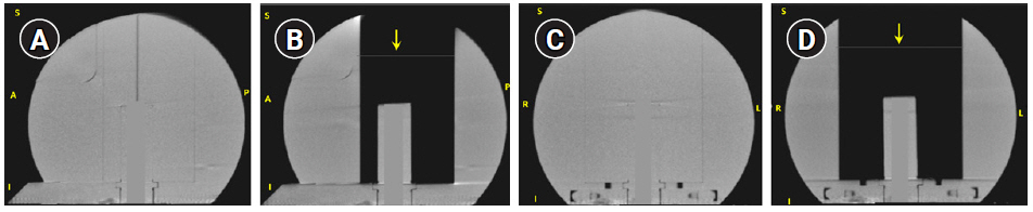
The TMR10 dose calculation was validated during commissioning by comparing dose planes measured by irradiating EBT3 films in the LGK solid water phantom (SWP) with corresponding DICOM RT-dose cubes exported from LGP via gamma analysis in a radiotherapy plan verification program. LGP’s convolution algorithm has been validated by multiple institutions [13]. To validate convCT and convCBCT, measurements were performed using an Exradin A1SL ion chamber in the SWP. The SWP is a spherical solid water phantom of radius 8 cm designed to be affixed to the Gamma Knife frame. The SWP has a higher attenuation coefficient than water at kilovoltage energies (due to higher Z-value), but similar electron density, leading to a discrepancy when the relative electron density of the phantom is calculated using a CT-ED curve based on tissue-equivalent materials. Fig. 2 shows the coronal and sagittal slices of the SWP with and without the central block. As LGP has no functionality to correct this discrepancy, the HU-value of the convCT and convCBCT datasets were estimated from a region-of-interest (contoured using Pinnacle³ TPS version 16.2.1) then the HU-values of the phantom were rescaled (using a Python script) so that the mean HU of the region-of-interest was equivalent to water (0 HU). In addition, HU values of the voxels corresponding to the chamber bore in the SWP were assigned a value of 0. A plan was created in LGP with a reasonably homogeneous dose distribution in the collecting volume of the detector. A structure (cylinder of 4 mm diameter and 4.2 mm length) approximating the collection volume of the detector was drawn, and the LGP calculated dose was defined as the mean dose to this structure. Plans were generated using TMR10, convCT and the convCBCT. These plans were then exported to the treatment console and delivered to the SWP. The dose measured with the A1SL ion chamber was compared to the LGP calculated dose. The dose difference D_Diff was defined as:

where D_LGP is the LGP calculated dose and D_Meas is the ion chamber measured dose.

To verify the accuracy of the convCT and convCBCT dose calculations in a non-uniform volume, the plans were recalculated on the SWP after removing a block of solid water from the phantom. The resulting phantom consists of the cylindrical chamber holder of a diameter 2.5 cm inside an air cavity of dimension 8.5 cm × 6.5 cm × 10 cm. The removed block included part of the superior surface of the phantom, it was necessary to add a surface structure to both CT datasets by replacing an 8.5 cm × 6.5 cm area of air in a single slice with low-density material (-450 HU), which was then classified as part of the skull by LGP.

A preliminary study was carried out with the CBCT to establish the relation between HU and the physical and electron densities of tissue equivalent materials. The CIRS Electron Density head phantom (Model 062M; CIRS) was imaged with the onboard CBCT of the Gamma Knife Icon. The phantom was imaged with water, adipose tissue, breast (50% adipose tissue, 50% glandular tissue), muscle, liver, lung (inhale), trabecular bone, and dense bone tissue. The phantom was imaged in two configurations to quantitatively assess any off-axis variation in HU in the cone beam. In the first configuration, the phantom was imaged at the center of the cone-beam FOV, with the inferior phantom edge being 9 cm from the edge mask adapter and aligned with the superior edge of the first flat surface for mask attachment. This position corresponded with the center of the phantom being 11.5 cm from the edge of the FOV in the longitudinal direction. In the second configuration, the phantom was imaged at the edge of the cone-beam FOV, with the inferior phantom edge aligned with the mask adapter. The phantom was imaged eight times in both configurations, with the phantom rotated by 45° between each measurement in order to assess the variation of HU with the angle. This corresponded to each insert being imaged at eight different angles (0°, 45°, 90°, 135°, 180°, -135°, -90°, and -45° relative to the 12 o'clock position). For each measurement, the central insert was set to be the same material as the insert at 0°. The central insert was used to relate the HU to the electron and physical densities of the material when the phantom was imaged at the center of the cone beam.

The CIRS Electron Density head phantom was also scanned in a Philips Brilliance Big Bore CT scanner (Philips Healthcare, Best, The Netherlands). The phantom was imaged twice in the center of the CT scanner’s FOV. The inserts were first imaged in the default configuration and then imaged with the phantom rotated by 180°, such that the inserts were located on the opposite side of the phantom compared to the first image. This allowed the calculation of the HU difference between the two orientations to assess off-axis variations in the planning CT images.

The convolution algorithm requires relative electron density data to be determined for each voxel in the planning dataset. A computed tomography number versus electron density (CT-ED) curve was determined for the Icon cone-beam CT using the average CT number measured at all positions for each insert in the CIRS Electron Density head phantom. CT-ED curves for CT datasets were based on previously commissioned clinical data based on measurements using the larger diameter Gammex 467 Tissue Characterization Phantom (Sun Nuclear Corporation, Melbourne, FL, USA). LGP does not extrapolate relative electron density values beyond the measured range of the CT-ED curve. Voxels with higher CT numbers than the maximum in the CT-ED curve are set to the electron density of the highest value within the curve, in this case corresponding to dense bone [11].

A retrospective set of 30 Gamma Knife treatment plans generated for patients with multiple brain metastases was selected. Of these plans, 12 targets were located in the frontal lobes, five targets in the temporal lobes, four in the parietal lobes, three in the cerebellum, two in the occipital lobes, and four targets in other sites. The clinical plans were generated with LGP version 11.1 using the TMR10 algorithm. Treatment plans were constructed following our departmental protocol, involving rigid co-registration of simulation CBCTs, CTs (if available) and MR images followed by contouring of target volumes and organs-at-risk. Shot arrangements were set up to cover the target, with iterative manual adjustments of shot weights and positions to optimize dose coverage and avoidance of normal tissue and limiting organs-at-risk. In addition, the prescription isodose (typically 50% of the maximum dose) can be adjusted to improve target coverage and selectivity. For plans with multiple targets, the cumulative dose was assessed and adjusted, if necessary. Each plan consisted of at least one target with at least two shots containing a target contour delineated by a radiation oncologist. Simulation CBCTs were used to define the outer contour of the skull and generate electron density information for treatment planning with the convolution algorithm. When available, planning CTs were also used for electron density data for treatment planning using the convolution algorithm. Treatment plans utilizing convolution algorithms on CBCT, and planning CT data were generated by changing the dose algorithm and electron density information used for calculations on the previously generated TMR10 plans. Treatment plans were evaluated using coverage, selectivity, gradient index, and beam-on time to assess changes introduced by using convolution using CBCT and planning CT data when compared to the TMR10 algorithm.

For dose measurements performed in the unmodified SWP, the difference in measured and LGP-calculated doses were -0.3%, -0.2%, and +1.8% when the dose was computed using TMR10, convCT, and convCBCT algorithms, respectively. The higher HU for the CBCT dataset is consistent with the expected higher photoelectric effect cross-section at the lower imaging energy (90 kV_p vs. 120 kV_p for the planning dataset). The higher discrepancy for the convCBCT dose calculation is assumed to be due to the non-uniformity in the HU of the CBCT datasets across the entire scanning volume and the uncertainty in the HU value scaling. For measurements in modified SWP with air cavity, where a block of solid water was removed from the SWP, the difference between measured and LGP calculated doses were -17.0%, -0.5%, and 1.4% for TMR10, convCT, and convCBCT, respectively. The TMR10 algorithm is expected to perform poorly as the air cavity is assigned the density of water. The results indicate that the convolution algorithms accurately model attenuation in this non-homogeneous phantom. Mean HU values of 29 HU and 304 HU for convCT and convCBCT, respectively and these values were used to rescale all voxels in each phantom dataset to a water equivalent relative electron density.

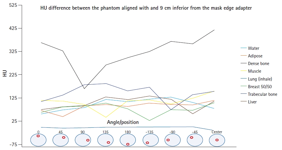
The HU measurements of the inserts imaged (mean ± standard deviation) with the CT and Icon CBCT scanners are shown in Table 1. The HU measurements in Table 1 were used in LGP for to generate CT-ED curves for use with Icon CBCT images. Fig. 3 shows the HU difference between the phantom aligned at the center of the cone beam and the inferior edge of the cone beam.

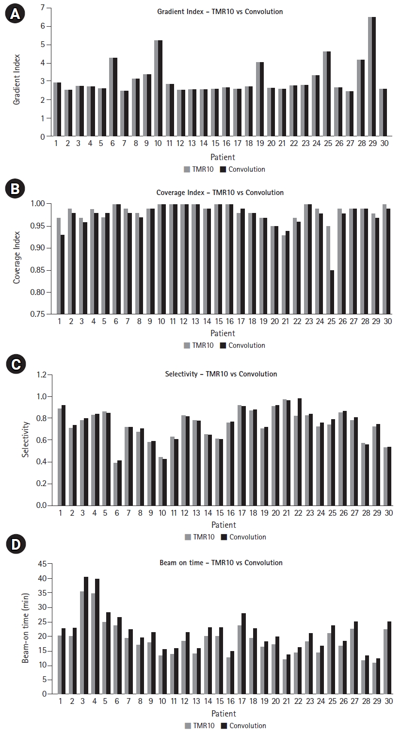
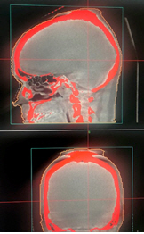
The mean coverage, selectivity, and gradient index was found to be 0.995 ± 0.008, 0.61 ± 0.13, and 3.3 ± 1.0 for convCT, respectively. Fig. 4 compares the mean coverage, selectivity, gradient index, and beam-on time of LGK treatment plans calculated with the TMR10 algorithm and with convCBCT, respectively. CBCT imaging with LGK Icon generates artifacts produced at the superior end of the scanner due to the non-symmetricity of the x-ray tube with the imaging panel is depicted in Fig. 5. Fig. 6 is a box and whisker plot of the mean calculated beam-on times for various treatment plans recalculated using TMR10, convCT, and convCBCT.

As seen in Fig. 3, the CT number of all the inserts in the CIRS phantom imaged with CBCT was observed to vary excessively with the insert’s position within the phantom. This was true whether the phantom was imaged in the center or at the edge of the cone-beam FOV. The greatest variation in HU (up to 408 HU) was seen for the dense bone insert when the CIRS phantom was imaged at the center of the cone-beam FOV. The average CT number of the inserts was also dependent on the position of the phantom within the cone-beam FOV, with the largest difference seen for dense bone. The difference in the average CT numbers of this insert when the phantom was imaged in the center and at the edge of the cone-beam FOV was 321 ± 195 HU. There were also large differences in the CT numbers of all other inserts of the CIRS phantom, with the exception of the lung (inhale) insert, where all measured values were near to the minimum HU value of -1000, representing an underestimate in electron density. As expected, the planning fan-beam CT image did not suffer the same HU variation issues as the CBCT.

The very significant changes in HU with respect to the insert position made it difficult to define a suitable CT-ED curve for dose calculations using CBCTs. As there was no way to encode positional variation in LGP’s CT-ED curve, the average CT number of all phantom measurements for each material were used. In addition, the density of dense bone was used as a cut-off value, with all materials with a higher HU set to this density. This was a deliberate choice to minimize the effect of the HU increase in the skull seen away from the center of the FOV in CBCT images and especially prominent at the superior end of the patient’s skull.

Typically, the convolution dose calculation algorithm in LGP uses electron density information from planning CT images. If CBCT images could be used instead, then planning CTs could be excluded from the workflow, as skull definition and electron density could be derived from the CBCT, with the target volume and organ-at-risk delineation performed on fused MRI images. As the CBCT is an integrated part of the Gamma Knife Icon and the whole system is calibrated to use the same stereotactic frame of reference, a high level of positional accuracy is ensured. Furthermore, as CBCT images are acquired with the patient on the treatment couch, the overall treatment process is greatly simplified. However, when using CBCT images for convolution dose calculations, the large variations in CT number and limited FOV must be taken into consideration, especially as the beam travels through the skull. It is imperative to ensure that this does not introduce any systematic dose calculation errors into the final treatment plan. Restricted acquisition angles tend to introduce a significantly higher density artifact at the superior edge of the skull. Such an artifact may be seen in the target coverage for patient #25, which decreased from 0.95 (TMR10) to 0.85 (convCBCT) (see Fig. 4).

In comparison, the measurements in the SWP indicated close agreement between dose and measurement for both convCT and convCBCT algorithms. It should be noted that convCBCT dose estimations at the center of the SWP are expected to be less affected by the two unfavorable influences observed on patient datasets: the target is at the center of the FOV. Therefore, the radiation contributing dose to the target will be attenuated by the full range of the HU-inhomogeneity, thus averaging out the influence of non-uniformity; secondly, the shots do not traverse the artifact at the superior apex of the phantom. This artifact is also reduced as the phantom is smaller than a typical human skull with no higher electron density material equivalent to the bone.

The coverage of Gamma Knife treatment plans generated using the TMR10 algorithm was 0.98 ± 0.02. The plan coverage achieved with convCBCT was 0.98 ± 0.03. Therefore, the choice to use the TMR10 or convolution algorithm with CBCT for treatment planning does not make a significant difference to the coverage of treatment plans (p = 0.13). This is reflected in the mean absolute difference in coverage between plans generated with the two different algorithms, which was 0.001.

The selectivity of Gamma Knife treatment plans generated using the TMR10 algorithm was 0.73 ± 0.14. The selectivity achieved with convCBCT was 0.75 ± 0.15. Therefore, the choice to use the TMR10 or convolution algorithm with CBCT for treatment planning does not make a significant difference to the selectivity of the treatment plans (p = 0.33). This is reflected in the mean absolute difference in selectivity between plans generated with the two different algorithms, which was 0.02.

The gradient index of Gamma Knife treatment plans generated using the TMR10 algorithm was 3.1 ± 0.94. The gradient index achieved with the convolution algorithm using CBCT images was 3.1 ± 0.97. Therefore, the choice to use the TMR10 or convolution algorithm with CBCT for treatment planning does not make a significant difference to the gradient index of treatment plans (p = 0.46). This is reflected in the mean absolute difference in gradient index between plans generated with the two different algorithms, which was 0.0002.

The results for coverage, selectivity, and gradient index are unsurprising because treating the patient as water equivalent will be an excellent approximation for most of the 192 beamlets for most shot positions.

Fig. 6 shows that planning treatments using convCBCT compared to TMR10 increased the average beam-on time from 18.9 ± 5.8 minutes to 21.7 ± 6.6 minutes. The choice of dose calculation algorithm therefore results in a significant increase in the beam-on time (p = 0.048). This was also observed when the plans were calculated with TMR10 and then recalculated with convCT (see Fig. 6). Moving from TMR10 to convCT increased the mean beam-on time by 6.9%. Moving from convCT to convCBCT increased the mean beam-on time by 8.6%. Overall, calculating the treatment plan using convCBCT instead of TMR10 increased the mean beam-on time by 16.2%.

There are three considerations that have a significant influence on the beam-on time. The first is the attenuation from the skull. Every beamlet in a shot will traverse the skull for almost all situations, lowering the dose rate at the shot position and thus increasing the beam-on time necessary. The second consideration is that HU values increase towards the edge of the FOV, introducing a spurious increase in necessary beam-on time. The third consideration is that high-density artifacts near the superior end of the skull in CBCT images may be traversed by beamlets, introducing another spurious increase in the beam-on time, particularly for superior targets. These considerations indicate that it is likely that the beam-on time calculated using convCT is more accurate than the underestimate calculated using TMR10 or the overestimate using convCBCT. It should be noted that a factor could potentially be applied to adjust the prescription dose based on the outcome data correlated to the treatment plans that have been historically calculated using TMR10 or similar homogeneous dose algorithms to correct for the increased beam-on time in the convCT algorithms.

A limitation of this study was that all plans considered were planned using TMR10 only. However, it should be noted that due to the practical limitations imposed by the calculation time, centers using the convolution algorithm will usually plan using TMR10 first, only using the convolution to make small iterative adjustments at the end of the plan construction.

In conclusion, the use of the convolution dose calculation algorithm with CBCT images for planning Gamma Knife treatment may offer benefits in terms of convenience and patient workflow. Regardless of this, it is clear that the total treatment time is increased by a mean value of over 16% compared to treatments calculated using the TMR10 algorithm. It is also clear that part of this increase is due to the limitations in the accuracy of the electron density information derived from CBCT images. The limitations of the CBCT imaging due to artifacts introduced by the small FOV and the large HU variation usually do not significantly impact the quality of the treatment plan in terms of coverage, selectivity, and gradient index. However, it is arguable that the limitations of CBCT-based electron density data may introduce more uncertainties into the dose algorithm for the limited benefit of incorporating heterogeneities into the dose calculation. Hence, the electron density data derived from the onboard CBCT should be used with caution. Scope for improvement may be found by processing CBCT images to segment them into electron densities for tissue, bone, and air.